11-5 SVM中使用多项式特征

import numpy as np
import matplotlib.pyplot as plt
from sklearn import datasets

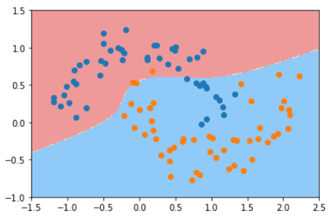
X, y = datasets.make_moons()
# X.shape = (100, 2)
# y.shape = (100,)

plot_decision_boundary(poly_svc, axis=[-1.5,2.5,-1.0,1.5])
plt.scatter(X[y==0,0],X[y==0,1])
plt.scatter(X[y==1,0],X[y==1,1])
plt.show()

X, y = datasets.make_moons(noise=0.15, random_state=666) # 0.15可以理解为标准差

plt.scatter(X[y==0,0],X[y==0,1])
plt.scatter(X[y==1,0],X[y==1,1])
plt.show()

使用多项式特征的SVM

训练模型

from sklearn.preprocessing import PolynomialFeatures, StandardScaler
from sklearn.svm import LinearSVC
from sklearn.pipeline import Pipeline

def PolynomialSVC(degree, C=1.0):
    return Pipeline([
        ('poly', PolynomialFeatures(degree=degree)),
        ('std_scaler', StandardScaler()),
        ('linearSVC', LinearSVC(C=C))
    ])

poly_svc = PolynomialSVC(degree=3)
poly_svc.fit(X, y)

绘制模型

def plot_decision_boundary(model, axis):
    x0, x1 = np.meshgrid(
        np.linspace(axis[0], axis[1], int((axis[1]-axis[0])*100)).reshape(-1,1),
        np.linspace(axis[2], axis[3], int((axis[3]-axis[2])*100)).reshape(-1,1)
    )
    X_new = np.c_[x0.ravel(), x1.ravel()]

    y_predict = model.predict(X_new)
    zz = y_predict.reshape(x0.shape)

    from matplotlib.colors import ListedColormap
    custom_cmap = ListedColormap(['#EF9A9A','#FFF59D','#90CAF9'])

    plt.contourf(x0, x1, zz, cmap=custom_cmap)

plot_decision_boundary(poly_svc, axis=[-1.5,2.5,-1.0,1.5])
plt.scatter(X[y==0,0],X[y==0,1])
plt.scatter(X[y==1,0],X[y==1,1])
plt.show()

使用多项式核函数的SVM

from sklearn.preprocessing import StandardScaler
from sklearn.svm import SVC
from sklearn.pipeline import Pipeline

def PolynomialKernelSVC(degree, C=1.0):
    return Pipeline([
        ('std_scaler', StandardScaler()),
        ('kernelSVC', SVC(C=C, kernel='poly', degree=degree))
    ])

poly_kernel_svc = PolynomialKernelSVC(degree=3)
poly_kernel_svc.fit(X, y)

plot_decision_boundary(poly_kernel_svc, axis=[-1.5,2.5,-1.0,1.5])
plt.scatter(X[y==0,0],X[y==0,1])
plt.scatter(X[y==1,0],X[y==1,1])
plt.show()