12-4 基尼系数
基尼系数的计算公式: 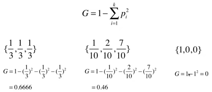 其性质与信息熵相同。
基尼系数越大,不确定性越高。
基尼系数越小,不确定性越低。
其性质与信息熵相同。
基尼系数越大,不确定性越高。
基尼系数越小,不确定性越低。
使用scikit learn中的基尼系数划分
import numpy as np
import matplotlib.pyplot as plt

from sklearn import datasets

iris = datasets.load_iris()
X = iris.data[:, 2:]
y = iris.target

from sklearn.tree import DecisionTreeClassifier

dt_clf = DecisionTreeClassifier(max_depth=2, criterion='gini')
dt_clf.fit(X, y)

def plot_decision_boundary(model, axis):
    x0, x1 = np.meshgrid(
        np.linspace(axis[0], axis[1], int((axis[1]-axis[0])*100)).reshape(-1,1),
        np.linspace(axis[2], axis[3], int((axis[3]-axis[2])*100)).reshape(-1,1)
    )
    X_new = np.c_[x0.ravel(), x1.ravel()]

    y_predict = model.predict(X_new)
    zz = y_predict.reshape(x0.shape)

    from matplotlib.colors import ListedColormap
    custom_cmap = ListedColormap(['#EF9A9A','#FFF59D','#90CAF9'])

    plt.contourf(x0, x1, zz, cmap=custom_cmap)

plot_decision_boundary(dt_clf, axis=[0.5, 7.5, 0, 3])
plt.scatter(X[y==0,0],X[y==0,1])
plt.scatter(X[y==1,0],X[y==1,1])
plt.scatter(X[y==2,0],X[y==2,1])
plt.show()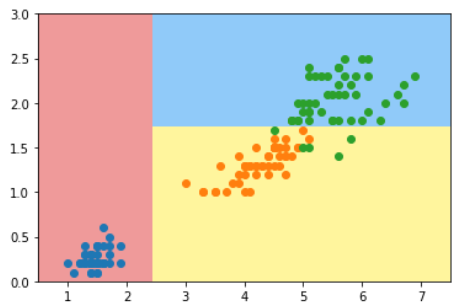
模拟使用基尼系数进行划分
信息熵 VS 基尼系数
Last updated