9-5 决策边界

如果X有两个特征，则 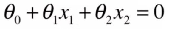决策边界为：

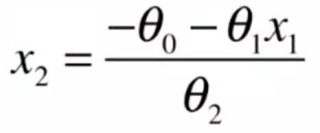
绘制决策边界

仍使用9-4中的例子

def x2(x1):
    return (-log_reg.coef_[0] * x1 - log_reg.interception_) / log_reg.coef_[1]

x1_plot = np.linspace(4, 8, 1000)
x2_plot = x2(x1_plot)

plt.plot(x1_plot, x2_plot)
plt.scatter(X[y==0,0],X[y==0,1], color='red')
plt.scatter(X[y==1,0],X[y==1,1], color='blue')
plt.show()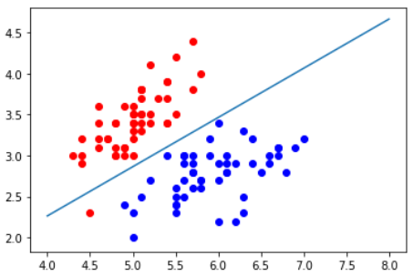

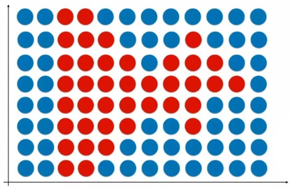
不规则的决策边界的绘制方法

def plot_decision_boundary(model, axis):
    x0, x1 = np.meshgrid(
        np.linspace(axis[0], axis[1], int((axis[1]-axis[0])*100)).reshape(-1,1),
        np.linspace(axis[2], axis[3], int((axis[3]-axis[2])*100)).reshape(-1,1)
    )
    X_new = np.c_[x0.ravel(), x1.ravel()]

    y_predict = model.predict(X_new)
    zz = y_predict.reshape(x0.shape)

    from matplotlib.colors import ListedColormap
    custom_cmap = ListedColormap(['#EF9A9A','#FFF59D','#90CAF9'])

    plt.contourf(x0, x1, zz, cmap=custom_cmap)

逻辑回归的决策边界

plot_decision_boundary(log_reg, axis=[4,7.5,1.5,4.5])
plt.scatter(X[y==0,0],X[y==0,1], color='red')
plt.scatter(X[y==1,0],X[y==1,1], color='blue')
plt.show()

KNN分类算法的决策边界

from sklearn.neighbors import KNeighborsClassifier

knn_clf = KNeighborsClassifier()
knn_clf.fit(X_train, y_train)

plot_decision_boundary(knn_clf, axis=[4,7.5,1.5,4.5])
plt.scatter(X[y==0,0],X[y==0,1], color='red')
plt.scatter(X[y==1,0],X[y==1,1], color='blue')
plt.show()

用KNN对三种iris进行分类的决策边界

knn_clf_all = KNeighborsClassifier()
knn_clf_all.fit(iris.data[:,:2], iris.target)

plot_decision_boundary(knn_clf_all, axis=[4,8,1.5,4.5])
plt.scatter(iris.data[iris.target==0,0],iris.data[iris.target==0,1], color='red')
plt.scatter(iris.data[iris.target==1,0],iris.data[iris.target==1,1], color='blue')
plt.scatter(iris.data[iris.target==2,0],iris.data[iris.target==2,1], color='green')
plt.show()

上图中，黄色与蓝色之间的边界存在过拟合

用KNN对三种iris进行分类的决策边界， K=50

knn_clf_all = KNeighborsClassifier(n_neighbors=50)
knn_clf_all.fit(iris.data[:,:2], iris.target)

plot_decision_boundary(knn_clf_all, axis=[4,8,1.5,4.5])
plt.scatter(iris.data[iris.target==0,0],iris.data[iris.target==0,1], color='red')
plt.scatter(iris.data[iris.target==1,0],iris.data[iris.target==1,1], color='blue')
plt.scatter(iris.data[iris.target==2,0],iris.data[iris.target==2,1], color='green')
plt.show()

KNN模型中，k值越大，模型越简单